Hodgkin-Huxley Model
The Hodgkin-Huxley model stands as a milestone in neuroscience, offering a comprehensive framework to comprehend the intricate dynamics of neuronal excitability. Developed by Sir Alan Lloyd Hodgkin and Sir Andrew Fielding Huxley in 1952, this model has been pivotal in shaping our understanding of how neurons generate and propagate electrical signals. In this blog post, we embark on a journey into the depths of the Hodgkin-Huxley neural model, exploring its inception, key components, and its profound impact on neuroscience.
The Birth of Hodgkin-Huxley Model:
The Hodgkin-Huxley model emerged as a result of pioneering experiments conducted on the giant axon of the squid. Hodgkin and Huxley meticulously studied the ion currents across the neuronal membrane, aiming to unravel the mechanisms underlying action potentials. Their groundbreaking work, which earned them the Nobel Prize in Physiology or Medicine in 1963, laid the foundation for the Hodgkin-Huxley model.
Understanding Neuronal Excitability:
The Hodgkin-Huxley model provides a mathematical description of the electrical activity in neurons. At its core, the model is based on the principles of ion channels and the flow of ions across the cell membrane. Sodium (Na+), potassium (K+), and leak channels play pivotal roles in shaping the dynamics of action potentials.
Components of the Hodgkin-Huxley Model:
Membrane Potential (Vm): The electric potential difference across the neuronal membrane. It is a dynamic variable influenced by ion currents and governs the excitability of the neuron.
Voltage-Gated Ion Channels (Na+, K+): Membrane structures that facilitate the transport of ions based on the membrane potential
- Sodium channels are responsible for the rapid influx of sodium ions during depolarization
- Potassium channels mediate the outward flow of potassium ions during repolarization
Leak Channels: Contribute to the resting membrane potential by allowing a continuous, passive flow of ions along the concentration gradient. While not as selective as voltage-gated channels, leak channels help maintain the baseline membrane potential.
Current ( $I_{\text{app}}, I_{\text{Na}}, I_{\text{K}}, I_{\text{L}}$): Movement of charged particles across a membrane. In this mode, there are four sources of current: Iapp which is externally applied to the neuron and the three currents produced by movement of ions through the sodium, potassium and leak channels described above.
Gating Variables (m, h, n): Gating variables represent the activation and inactivation states of sodium and potassium channels.
- m represents the activation of sodium channels.
- h represents the inactivation of sodium channels.
- n represents the activation of potassium channels.
Transition Rate Constanst (α, β): These factors guide the dynamics of ion channel state changes.
- α is the number of times per second that a gate which is in the shut state opens
- β is the number of times per second that a gate which is in the open state shuts
Mathematical Formulation:
The model’s equations involve differential equations that use Euler’s method to describe the changes in membrane potential and ion concentrations over time. These equations elegantly capture the complex interplay between ion channels, enabling simulations of action potentials under various conditions.
Membrane Potential Equation
$$ C_m \frac{dV}{dt} = I_{\text{app}} + I_{\text{Na}} + I_{\text{K}} + I_{\text{L}} $$Sodium Current Equation
$$ I_{\text{Na}} = g_{\text{Na}}m^3h(E_{\text{Na}} - V_m) $$Potassium Current Equation
$$ I_{\text{K}} = g_{\text{K}}n^4(E_{\text{K}} - V_m) $$Leak Current Equation
$$ I_{\text{L}} = g_{\text{L}}(E_{\text{L}} - V_m) $$Gating Variables Equations
$$ \frac{dm}{dt} = \alpha_m(1 - m) - \beta_mm $$ $$ \frac{dh}{dt} = \alpha_h(1 - h) - \beta_hh $$ $$ \frac{dn}{dt} = \alpha_n(1 - n) - \beta_nn $$Alpha $(\alpha)$ and Beta $(\beta)$ Formulas
\begin{align*}
\text{For } m: & \quad \alpha_m = \frac{10^5 (-V_m - 0.045)}{\exp(100 (-V_m - 0.045)) - 1} \\
& \quad \beta_m = 4 \times 10^3 \exp\left(\frac{-V_m - 0.070}{0.018}\right) \\
\\
\text{For } h: & \quad \alpha_h = 70 \exp(50 (-V_m - 0.070)) \\
& \quad \beta_h = \frac{10^3}{\exp(100 (-V_m - 0.040)) + 1} \\
\\
\text{For } n: & \quad \alpha_n = \begin{cases} 100 & \text{if } V_m = -0.060 \\ \frac{10^4 (-V_m - 0.060)}{\exp(100 (-V_m - 0.060)) - 1} & \text{otherwise} \end{cases} \\
& \quad \beta_n = 125 \exp\left(\frac{-V_m - 0.070}{0.08}\right) \\
\end{align*}
Note: The if statement applies L'Hôpital's rule to calculate $\alpha_n$.
function HodgkinHuxley()
    % This is a famous neuron model developped by Hodgkin and Huxley
    % There are four time-dependent variables: sodium activation, sodium inactivation,
    % potassium activation, and membrane potential


    % Default model parameters
    Gl = 3*10^-8; % Leak Conductance (S)
    Gna = 1.2*10^-5; % Maximum Sodium Conductance (S)
    Gk = 3.6*10^-6; % Maximum Delayed Rectifier Conductance (S)
    Ena = 4.5*10^-2; % Sodium Reversal Potential (V)
    Ek = -8.2*10^-2; % Potassium Reversal potential (V)
    El = -6*10^-2; % Leak Reversal potential (V)
    Cm = 10^-10; % Membrane capacitance (F)

    % Initial conditions
    conditions = [El 0 0 0]; % [Vm m h n]

    % Default simulation parameters
    tmax = 0.35; % Duration of trial
    delta = 0.00001; % Step size
    nSteps = int32((tmax)/delta); % Number of steps in a simulation
    Iapp = zeros(1,nSteps+1); % Applied current throughout the trial

    % This function calculates rate constants based on the value of Vm
    function constants = gatingVariables(Vm)
        % Gating variable m
        % Steady state: Am / (Am + Bm)
        % Time constant: 1 / (Am + Bm)
        Am = (10^5 * (-1 * Vm - 0.045))/(exp(100 * (-1 * Vm - 0.045)) - 1);
        Bm = 4 * 10^3 * exp((-1 * Vm - 0.070)/0.018);

        % Gating variable h
        % Steady state: Ah / (Ah + Bh)
        % Time constant: 1 / (Ah + Bh)
        Ah = 70 * exp(50 * (-1 * Vm - 0.070));
        Bh = 10^3 / (exp(100 * (-1 * Vm - 0.040)) + 1);

        % Gating variable n
        % Steady state: An / (An + Bn)
        % Time constant: 1 / (An + Bn)
        if Vm == -0.060 % L'Hopital's rule used to calculate An in the case it is 0/0
            An = 100;
        else
            An = (10^4 * (-1 * Vm - 0.060))/(exp(100 * (-1 * Vm - 0.060)) - 1);
        end
        Bn = 125 * exp((-1 * Vm - 0.070)/0.08);
        constants = [Am Bm Ah Bh An Bn];
    end

    % Differential Equations for the Hodgkin Huxley Model
    function rates = differentialEquations(Vm,Iapp,m,h,n)
        constants = gatingVariables(Vm);
        dVm = (Gl * (El - Vm) + Gna * m^3 * h * (Ena - Vm) + Gk * n^4 * (Ek - Vm) + Iapp)/Cm;
        dm = constants(1) * (1-m) - constants(2) * m;
        dh = constants(3) * (1-h) - constants(4) * h;
        dn = constants(5) * (1-n) - constants(6) * n;
        rates = [dVm dm dh dn];
    end

    % This function simulates one trial and returns various data in a cell
    function data=simulate(delta,nSteps,Iapp,conditions)
        % Gather initial conditions
        Vm = conditions(1);
        m = conditions(2);
        h = conditions(3);
        n = conditions(4);

        % Initialize several data vectors and add first values
        VmData = zeros(1,nSteps+1);
        mData = zeros(1,nSteps+1);
        hData = zeros(1,nSteps+1);
        nData = zeros(1,nSteps+1);
        VmData(1) = Vm;
        mData(1) = m;
        hData(1) = h;
        nData(1) = n;

        % This for loop iterates for each time point in the experiment
        for j=2:nSteps+1
            rates = differentialEquations(Vm,Iapp(j),m,h,n);
            Vm = Vm + (rates(1) * delta);
            m = m + (rates(2) * delta);
            h = h + (rates(3) * delta);
            n = n + (rates(4) * delta);

            % Several pieces of data are recorded
            VmData(j) = Vm;
            mData(j) = m;
            hData(j) = h;
            nData(j) = n;
        end
        % The data is packaged into a cell array
        data = {VmData,mData,hData,nData};

        % Values are reset to baseline at the end of the simulation
        Vm = conditions(1);
        m = conditions(2);
        h = conditions(3);
        n = conditions(4);
    end
end
The default conditions listed above simulate the following neural activity.
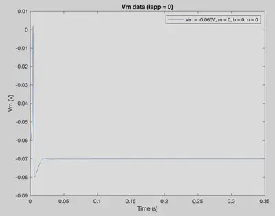
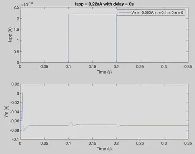
By changing initial conditions and the pattern of applied current (Iapp), various firing patterns can be produced.
tmax = 0.35; % Duration of trial
delta = 0.00001; % Step size
nSteps = int32((tmax)/delta); % Number of steps in simulation
Iapp = zeros(1,nSteps+1); % Applied current throughout the trial
Iapp(0.1/delta:0.2/delta) = 2.2*10^-10;
conditions = [El 0 0 0]; % [Vm m h n]
tmax = 0.35; % Duration of trial
delta = 0.00001; % Step size
nSteps = int32((tmax)/delta); % Number of steps in simulation
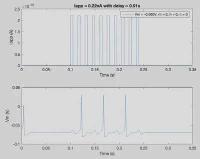
% The following several lines of code produce a unique Iapp
% pattern with 10 excitatory pulses
Iapp = zeros(1,nSteps+1); % Applied current throughout the trial
delay = 0.01; % Delay variable that influences timing of current
IappPattern = [];
for i=1:10
temp1 = ones(1,int32(0.005/delta))*2.2*10^-10;
temp2 = zeros(1,int32(delay/delta));
IappPattern = cat(2,IappPattern,temp1);
IappPattern = cat(2,IappPattern,temp2);
end
Iapp(int32(0.1/delta):(int32(0.1/delta)+size(IappPattern,2)-1)) = IappPattern;
conditions = [El 0 0 0]; % [Vm m h n]
tmax = 0.35; % Duration of trial
delta = 0.00001; % Step size
nSteps = int32((tmax)/delta); % Number of steps in simulation
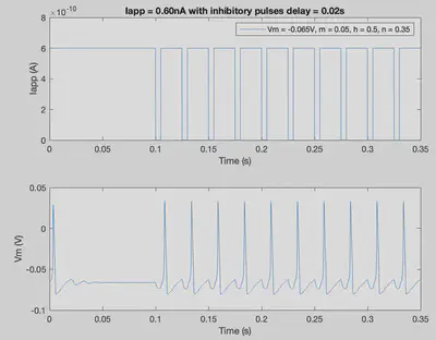
delay = 0.020; % Delay is set to 20ms
% The following several lines of code produce a unique Iapp
% pattern with 10 inhibitory pulses
Iapp = ones(1,nSteps+1)*6.0*10^-10; % Applied current throughout the trial
IappPattern = [];
for i=1:10
temp1 = zeros(1,int32(0.005/delta));
temp2 = ones(1,int32(delay/delta))*6.0*10^-10;
IappPattern = cat(2,IappPattern,temp1);
IappPattern = cat(2,IappPattern,temp2);
end
Iapp(0.1/delta:((0.1/delta)+size(IappPattern,2)-1)) = IappPattern;
conditions = [-0.065 0.05 0.5 0.35]; % [Vm m h n]
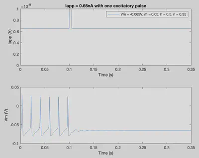
tmax = 0.35; % Duration of trial
delta = 0.00001; % Step size
nSteps = int32((tmax)/delta); % Number of steps in simulation

Iapp = ones(1,nSteps+1)*6.5*10^-10; % Applied current throughout the trial
Iapp(int32(0.1/delta):int32(0.105/delta)) = 10^-9; % One excitatory pulse
conditions = [-0.065 0.05 0.5 0.35]; % [Vm m h n]
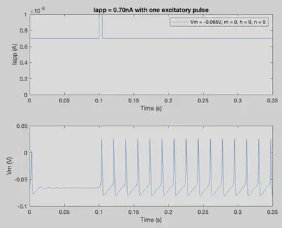
tmax = 0.35; % Duration of trial
delta = 0.00001; % Step size
nSteps = int32((tmax)/delta); % Number of steps in simulation

Iapp = ones(1,nSteps+1)*7.0*10^-10; % Applied current throughout the trial
Iapp(int32(0.1/delta):int32(0.105/delta)) = 10^-9; % One excitatory pulse
conditions = [-0.065 0 0 0];
Impact on Neuroscience:
The Hodgkin-Huxley model has had a profound impact on neuroscience and computational neuroscience in particular. It serves as a cornerstone for studying neuronal excitability, guiding research in diverse areas such as synaptic transmission, neural networks, and neuropharmacology.
Challenges and Extensions:
While the Hodgkin-Huxley model provides a robust foundation, it is not without limitations. Simplifications and assumptions made in the model’s development open avenues for deviations from neural activity in the real world. Modern computational models often build upon Hodgkin-Huxley principles, incorporating additional features that attempt to more closely replicate neural morphology and behavior.
Max Melnikas
Master of Science Candidate
My research interests include applications of digital devices for cognitive health monitoring and research matter.